
Class 11-commerce NCERT Solutions Economics Chapter 4: The Theory of the Firm under Perfect Competition
The Theory of the Firm under Perfect Competition Exercise 67
Solution 1
A perfectly competitive market is a type of market where there are a large number of buyers and sellers. Characteristics of a perfectly competitive market:
Large number of sellers and buyers: The main feature of a perfectly competitive market is a large number of buyers and sellers in the market. Due to this feature, no single buyer or seller can influence market prices.
Homogeneity: All the producers in a perfectly competitive market always produce a similar type of products. Homogeneity in products is one of the important features of a perfectly competitive market.
Complete mobility of factors of production: In a perfectly competitive market, all the factors of production can shift from one place to another for better opportunity purposes.
No transportation cost: All the goods and services are manufactured in a local market, so transportation cost exists in a perfectly competitive market.
Free exit and entry: All the firms in a perfectly competitive market can enter and exit from the market according to their wish in the long run. In the short run, it becomes difficult for firms to enter and exit from the market.
No selling cost: Selling cost does not exist in a perfectly competitive market.
Perfect knowledge of the market: The main characteristic of a perfectly competitive market is that all the buyers and sellers have perfect knowledge about the market, especially about the prices and quality of products sold in the market.
Solution 2
Total revenue is measured by considering the price of goods and the total quantity sold in the market.
The following formula is used to calculate the total revenue:
![]()
Market price and marginal revenue are the same in a perfectly competitive market as both forms are price takers. The price is determined by market forces (i.e. market demand and market supply).
Firms can increase their total revenue by selling more quantity of goods and services as the price of products cannot be changed by them.
Solution 3
The price line is the line that represents the graphical relationship between price and output. The demand curve and the price line are equal in a perfectly competitive market.
Graphical representation of the price line:
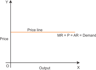
The line indicates that a firm can sell its goods and services at the existing price. The shape of the price line in a perfectly competitive market is horizontal.
Solution 4
The total revenue curve of a price-taking firm is an upward-sloping straight line because of the following reasons:
- The average revenue remains constant at all stages of production in a perfectly competitive market.
- The price of products remains constant in a perfectly competitive market.
- Average revenue is equal to the marginal revenue in a perfectly competitive market.
- All the firms are price takers.
The total revenue curve passes through its origin because no revenue will be generated if the output sold is zero. The revenue will be generated only when the output is sold.
The Theory of the Firm under Perfect Competition Exercise 68
Solution 5
Total revenue is calculated by considering the price and the quantity sold. Average revenue is calculated by considering the total revenue and the quantity sold.

Hence, in a perfectly competitive market, the average revenue and the price of products are equal. The average changes according to changes in price.
Solution 6
Marginal revenue is the revenue which is generated by selling an additional unit of a commodity. It is the change in total revenue when an additional unit of a commodity is sold in the market.
The relationship between market price and marginal revenue can be explained by using the following equations:

TR = Total revenue
MR = Marginal revenue
Q = Quantity
![]()
The above equation indicates that the price is equal to marginal revenue in a perfectly competitive market.
Graphical representation of the relationship between marginal revenue and price:
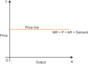
The diagram shows that the price, marginal revenue, average revenue and demand curve are the same in a perfectly competitive market.
Solution 7
If a profit-maximising firm produces positive output in a competitive market, then the following conditions must hold:
At the quantity level, marginal revenue should be equal to marginal cost. If the marginal revenue is less than the marginal cost, then a firm would not produce more quantity in a perfectly competitive market.
There should be an increase in the marginal cost according to an increase in the quantity produced.
Price should not be less than the average variable cost. It should be equal or greater than that of the price in short run.
Price should not be less than the long-run average cost. The price should be equal or more than the long-run average cost.
Solution 8
It is merely impossible for a profit-maximising firm to produce a positive level of output at which the market price is not equal to the marginal cost.
If the marginal cost is greater than the market price, then the producer will stop producing goods to avoid losses.
If the price is greater than the marginal cost, then a firm will not make positive profit. A firm has to reduce its output to make the profit.
Graphical representation of the marginal cost:
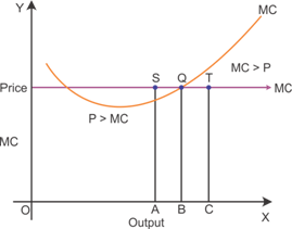
The diagram shows that a profit-maximising firm cannot produce a positive level of output if the marginal cost is not equal to the market price. A firm can produce a positive level of output when the marginal cost is equal to the market price as indicated in the diagram.
Solution 9
It is merely impossible for a profit-maximising firm to produce a positive level of output in the range where the marginal cost is decreasing.
According to the conditions of a profit-maximising firm, the marginal cost should be upward sloping or it should be equal to the market price.
Graphical representation indicating the behaviour of the marginal cost curve:
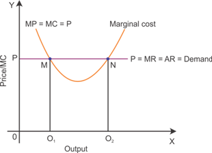
The diagram shows the behaviour of the marginal cost curve. The diagram indicates that the profit can only be maximised when the marginal cost is equal to the market price. If the marginal cost of a firm is less than the market price, then a firm will not make positive profit. A firm has to reduce its output to make profit.
Solution 10
It is merely impossible for a profit-maximising firm to produce a positive level of output in the short run if the market price is less than the minimum of AVC.
If the average variable cost is greater than the market price, then the producer will stop producing goods to avoid losses.
Firms will have to incur losses if the price is less than the minimum of the average cost.
Graphical representation indicating the behaviour of the average variable cost:
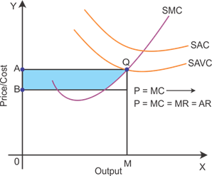
The diagram indicates the losses which a firm has to incur if it keeps on producing goods and services even if the price falls below the minimum of average variable cost. The shaded area in the above diagram indicates losses.
Solution 11
A profit-maximising firm in a competitive market will not produce a positive level of output in the long run if the market price is less than the minimum of AC because of free entry and exit from the market in the long run.
If the price is less than that of the minimum of average cost, then firms will have to incur losses.
All the firms in a competitive market earn zero economic profit. So, if the price becomes less than the minimum of average cost, then they will stop production to avoid losses.
Graphical representation indicating the behaviour of long-run average cost:
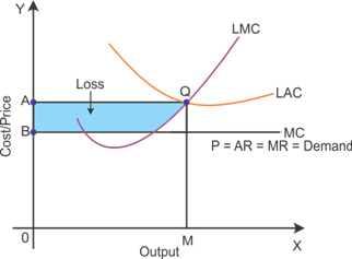
The diagram indicates the losses which a firm has to incur if it keeps on producing goods and services even if the price falls below the minimum of average cost in the long run. The shaded area in the diagram indicates losses.
Solution 12
The upward sloping part of the short-run marginal cost curve is considered the supply curve of a firm in the short run.
The supply curve of a firm in the short run is comparatively less elastic as it cannot be changed according to changes in the demand for goods and services. The supply curve is also regarded as the addition of the upward sloping portion of short-run marginal cost.
Graphical representation indicating the supply curve in the short run:
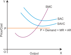
The diagram indicates the upward sloping part of the marginal cost curve which is considered the short run supply curve of a firm in the short run.
Solution 13
In the long run, supply of goods and services can be changed according to the changes in the demand. So, the shape of the supply curve in the long run is elastic as indicated in the diagram.
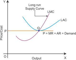
The supply curve is upward sloping with an addition of the rising long-run marginal cost curves.
Solution 14
Technological progress reduces the marginal cost of production. Producers can produce comparatively more goods and services with the help of available factors of production. This situation is likely to shift the supply curve rightward and the marginal cost curve downward.
There is a positive relationship between technological progress and supply. Technological progress often leads to a decline in the cost of production which enables producers to produce and supply more goods and services at the existing price.
Thus, technological progress is likely to increase supply causing a rightward shift in the supply curve.
Solution 15
A unit tax is the tax imposed on the per unit sold quantity. Imposition of a unit tax increases the cost of production per unit. This finally raises the marginal cost. Rise in the marginal cost leads to a decline in the supply causing a leftward shift in the supply curve.
An imposition of taxes creates additional burden on the burden causing a rise in the cost of production. Sometimes, producers increase the price of goods and services to reduce the burden of taxes. A rise in the price again causes a decline in the demand. A decline in demand reduces the supply.
Thus, the imposition of a unit tax is likely to decrease the supply causing a leftward shift in the supply curve.
Solution 16
An increase in the price of an input causes a rise in the cost of production. The marginal cost tends to increase due to a rise in the cost of production. Rise in the marginal cost leads to a decline in the supply causing a leftward shift in the supply curve.
An increase in the price of inputs leads to rise in the cost of production. Sometimes, producers increase the price of goods and services to reduce the burden of additional cost. A rise in the price again causes a decline in the demand. Decline in demand reduces the supply.
Thus, an increase in the price of an input is likely to decrease the supply causing a leftward shift in the supply curve.
Solution 17
The market supply curve is likely to shift rightward due to an increase in the number of firms in a market.
An increase in the number of firms in the market causes an increase in the total supply. An increase in the total supply causes a rightward shift in the supply curve. The market supply curve is derived adding all the individual supply curves in the market.
Solution 18
Price elasticity of supply is the percentage change in the quantity supplied for a good divided by the percentage change in the price of that particular good.
![]()
Price elasticity of supply indicates the responsiveness of the quantity supplied to changes in the price. The following formula is used to measure the price elasticity of supply:
Solution 19
Total revenue is calculated by considering the price of a good and the total quantity sold. Marginal revenue is the revenue generated by selling an additional unit of a commodity. It is the change in total revenue when an additional unit of a commodity is sold in the market.
Total revenue, marginal revenue and average revenue are computed in the table below:
|
Quantity sold |
Total Revenue |
Marginal Revenue |
Average Revenue |
|
0 |
- |
- |
- |
|
1 |
10 |
10 |
10 |
|
2 |
20 |
10 |
10 |
|
3 |
30 |
10 |
10 |
|
4 |
40 |
10 |
10 |
|
5 |
50 |
10 |
10 |
|
6 |
60 |
10 |
10 |
Solution 20
The profit at each output level is calculated by considering the total revenue and the total cost. The market price is calculated by considering the total revenue and the quantity. Market price and profitability are determined in the following table:
|
Quantity Sold |
Total Revenue |
Total Cost |
Profit |
Market Price=
|
|
0 |
0 |
5 |
-5 |
- |
|
1 |
5 |
7 |
-2 |
5 |
|
2 |
10 |
10 |
0 |
5 |
|
3 |
15 |
12 |
3 |
5 |
|
4 |
20 |
15 |
5 |
5 |
|
5 |
25 |
23 |
2 |
5 |
|
6 |
30 |
33 |
-3 |
5 |
|
7 |
35 |
40 |
-5 |
5 |

The above table shows that the market price is determined at the level of 5. The average revenue remains the same across all the units as there is constant increase in the total revenue.
The Theory of the Firm under Perfect Competition Exercise 69
Solution 21
The profit at each output level is calculated by considering the total revenue and the total cost. Total cost is deducted from the total revenue to calculate the profit at each level of output as indicated in the table below.
|
Quantity Sold |
Total Cost |
Price |
Profit |
Total revenue |
|
0 |
5 |
10 |
-5 |
0 |
|
1 |
15 |
10 |
-5 |
10 |
|
2 |
22 |
10 |
-2 |
20 |
|
3 |
27 |
10 |
3 |
30 |
|
4 |
31 |
10 |
9 |
40 |
|
5 |
38 |
10 |
12 |
50 |
|
6 |
49 |
10 |
11 |
60 |
|
7 |
63 |
10 |
7 |
70 |
|
8 |
81 |
10 |
-1 |
80 |
|
9 |
101 |
10 |
-11 |
90 |
|
10 |
123 |
10 |
-23 |
100 |
The profit-maximising level of output is determined at the level where a producer is earning maximum profit. As shown in the above table, the maximum profit 12 is earned by selling 5 units of a quantity. Thus, the profit-maximising level of output is 5 units.
Solution 22
The market supply schedule is a summation of individual supply schedules in the market. The market supply can be calculated by adding all the individual supply schedules in the market as indicated in the table below.
|
Price |
SS1 (Units) |
SS2 (Units) |
Market Supply |
|
0 |
0 |
0 |
0 |
|
1 |
0 |
0 |
0 |
|
2 |
0 |
0 |
0 |
|
3 |
1 |
1 |
2 |
|
4 |
2 |
2 |
4 |
|
5 |
3 |
3 |
6 |
|
6 |
4 |
4 |
8 |
Solution 23
The market supply schedule is a summation of individual supply schedules in the market. The market supply can be calculated by adding all the individual supply schedules in the market as indicated in the table below.
|
Price |
SS1 (Kg) |
SS2 (Kg) |
Market Supply |
|
0 |
0 |
0 |
0 |
|
1 |
0 |
0 |
0 |
|
2 |
0 |
0 |
0 |
|
3 |
1 |
0 |
1 |
|
4 |
2 |
0.5 |
2.5 |
|
5 |
3 |
1 |
4 |
|
6 |
4 |
1.5 |
5.5 |
|
7 |
5 |
2 |
7 |
|
8 |
6 |
2.5 |
8.5 |
Solution 24
Identical firms have similar type of supply schedules. The supply schedule of the other two firms is shown in the following table:
|
Price |
SS1 (Units) |
SS2 (Units) |
SS3 (Units) |
Market Supply |
|
0 |
0 |
0 |
0 |
0 |
|
1 |
0 |
0 |
0 |
0 |
|
2 |
2 |
2 |
2 |
6 |
|
3 |
4 |
4 |
4 |
12 |
|
4 |
6 |
6 |
6 |
18 |
|
5 |
8 |
8 |
8 |
24 |
|
6 |
10 |
10 |
10 |
30 |
|
7 |
12 |
12 |
12 |
36 |
|
8 |
14 |
14 |
14 |
42 |
Market supply is calculated by adding all the individual supply schedules in the market.
The Theory of the Firm under Perfect Competition Exercise 70
Solution 25
As given,
Revenue = 50
Market price of a good = 10
At the price of Rs. 10, the total revenue earned is 50 units. So, the quantity sold is 5 units as the total revenue is calculated by multiplying the quantity sold and the price.
Hence,
Quantity sold at price 10 is 5 units.
At the price of Rs. 15, the total revenue earned is 150 units. So, the quantity sold is 10 units as the total revenue is calculated by multiplying the quantity sold and the price.
Quantity sold at price 15 is 10 units.
Elasticity of supply is calculated by considering the change in quantity and the change in price. The following formula is used to calculate the elasticity of supply:


The price elasticity of the firm's supply curve is 2.
Solution 26
As given,
Elasticity of supply = 0.5
Final price = 20
Initial price = 5
Change in quantity = 15
The change in price can be calculated by deducting the initial price from the final price.

Putting the above values in the formula of elasticity of supply,

Thus, the initial level of output is 10 units. As the quantity is increased by 15 units, the final level of output would be 10 + 15 = 25.
Solution 27
As given,
Initial market price = 10
Final market price = 30
Quantity supplied = 4 units
The price elasticity of the firm's supply = 1.25
The change in price can be calculated by deducting the initial price from the final price.

Putting the above values in the formula of elasticity of supply,

So, the change in quantity of output is 10 units. The new quantity which will be supplied with the new price can be calculated by adding the change in quantity in the initial price.

Thus, with the new price, the firm will supply 14 units.