
Class 11-commerce NCERT Solutions Economics Chapter 3: Production and Costs
Production and Costs Exercise 50
Solution 1
The production function of a firm describes the relationship between the output and the factors of production which are being used in the production process. It shows the required number of inputs needed to produce the maximum level of final output.
The following formula is used to express the production function:
![]()
where
Q = final units of output
![]()
The above equation shows that the final units of output can be produced by using production factors 1 and 2.
Solution 2
Total product is the summation of the final units of output produced by a firm by using the given amount of inputs during a particular period of time.
Total product is the relationship between variable factors of production and final units of output when all other factors of production are held constant. The following formula can be used to express the total product:
Total Product = ![]()
The above formula shows the relationship between variable factors of production and the summation of the total output.
Solution 3
Average product is the output per unit of variable input. It indicates the ratio of the total product by variable factors of production. The following formula can be used to describe the average product:
![]()
Solution 4
Marginal product of an input is the change in the total output caused by the changes in the variable inputs when other inputs are held constant.
It is calculated by considering the additional change in the total units of output due to changes in employing the additional units of variable inputs. The following formula can be used to describe the marginal product of an input:
Marginal Product of an Input
= Change in Total Product/Change in Variable Product
Solution 5
Total product of an input rises at an increasing rate when there is an increase in the marginal product. The relationship between the marginal product and the total product of an input can be explained with the following diagrammatic representation:
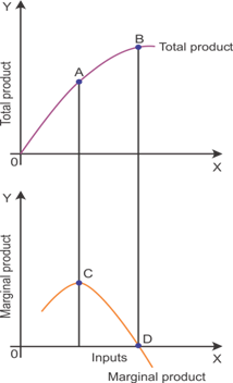
The diagram shows that the total product increases at an increasing rate when there is an increase in the marginal product.
Total product increases after Point A but at a decreasing rate due to a decline in the marginal product. The marginal product curve starts diminishing after Point C.
Total product is at its maximum level at Point B when the marginal product is zero at Point D.
Total product starts decreasing when the marginal product becomes negative.
Solution 6
Short run: Short run is the period in which all the factors of production cannot be changed to change the output. In a short run, the output cannot be increased by increasing both variable factors and fixed factors of production. Firms cannot change the fixed factors of production in the short run.
Output in the short run can only be changed by changing the variable factors of production.
Long run: Long run is the period in which all the factors of production can be changed to change the output. In a long run, the output can be increased by increasing both variable factors and fixed factors of production. Firms can change fixed factors of production in the long run.
Output in the long run can be changed by changing the variable and fixed factors of production.
Solution 7
According to the law of diminishing marginal product, the marginal product tends to diminish when more and more units of variable factors of production are used in the production process.
At the initial stage, the marginal product increases at an increasing rate, but when more variable inputs are used in the production, the marginal product keeps on decreasing.
Excessive use of variable inputs can lead to negative marginal product.
Solution 8
Definition of law of variable proportions according to Samuelson:
An increase in some inputs relative to other fixed inputs will in a given state of technology cause output to increase, but after a point, the extra output resulting from the same additions of extra inputs will become less and less.
The law of variable proportions indicates the relationship between the units of variable factors of production and the output in the short run.
Excessive use of variable factors of production can lead to zero or negative addition to the total product.
Solution 9
Constant returns to scale is satisfied when there is equal changes in the factors of production and the changes in output. The main criterion for constant returns to scale is proportionate changes in inputs and the final output.
If there are unequal changes in the inputs and outputs, then the constant returns to scale cannot be achieved.
For example, constant returns to scale is satisfied when an increase in factors of production by 25% causes an increase in the final output by 25%.
Solution 10
Increasing returns to scale is satisfied when an increase in the factors of production leads to more than proportionate increase in the final output. The main criterion for increasing returns to scale is higher proportionate changes in final outputs than inputs.
If there are equal changes in the inputs and outputs, then the increasing returns to scale cannot be achieved.
For example, increasing returns to scale is satisfied when an increase in factors of production by 25% causes an increase in the final output by 35%.
Production and Costs Exercise 51
Solution 11
Decreasing returns to scale is satisfied when an increase in the factors of production leads to less than proportionate increase in the final output. The main criterion for decreasing returns to scale is lower proportionate changes in final outputs than inputs.
If there are equal changes in the inputs and outputs, then the decreasing returns to scale cannot be achieved.
For example, decreasing returns to scale is satisfied when an increase in factors of production by 25% causes an increase in the final output by 15%.
Solution 12
The cost function is described as the functional relationship between the cost of production and the output. The cost function can be expressed by the following formula:
![]()
![]()
The above formula indicates the relationship between cost and final output. Changes to the cost of production are likely to change the final output.
Solution 13
Total fixed cost: Total fixed cost is the cost incurred by producers for acquiring fixed factors of production. For example, the cost of buying machinery and building can be considered the total fixed cost. Total fixed cost cannot be changed in the short run.
Total variable cost: Total variable cost is the cost incurred by producers for acquiring variable factors of production. For example, the cost of buying labour can be considered the total variable cost. Total variable cost can be changed in the short run.
Total cost: Total cost is the summation of the total variable cost and the total fixed cost. For example, the cost of buying labour, machinery and building can be considered total cost.
The total cost changes because of changes in total variable cost and total fixed cost.
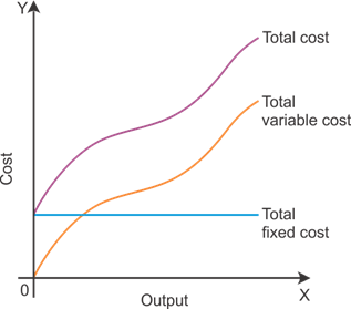
Relationship between total fixed cost, total variable cost and total cost
Total cost increases due to changes in the variable cost.
Fixed cost remains constant as there is no change in the fixed factors of production.
Total fixed cost is the main difference between total cost and total variable cost.
There is a proportionate increase in the total variable cost and total cost.
Solution 14
Average fixed cost: Average fixed cost is the per unit fixed cost of production. It is calculated by using the following formula:
![]()
Average variable cost: Average variable cost is the per unit variable cost of production. It is calculated by using the following formula:
![]()
Average cost: Average cost is the per unit total cost of production. It is calculated by using the following formula:
![]()
Relationship between average variable cost, average fixed cost and average cost: Average cost can be calculated by considering the average variable and average fixed cost. An increase in the average variable cost and average fixed cost causes an increase in the average cost.
Solution 15
There cannot be some fixed cost in the long run as it only occurs in the short run. In the long run, all the factors of production are variable and they can be changed according to the requirement.
Fixed factors in the short run become variables factors in the long run. Producers get enough time to change the factors of production in order to change production.
Thus, fixed cost does not exist in the long run.
Solution 16
The average fixed cost is the per-unit fixed cost of production. The shape of the average fixed cost curve is a rectangular hyperbola.
This is because AFC falls with an increase in output as TFC is same at all levels of output. Due to this, the average fixed cost curve slopes downward from left to right.
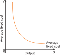
Average fixed cost curve
The above diagram shows that the average fixed cost tends to diminish as there is an increase in the output.
Solution 17
The short run marginal cost, average variable cost and short run average cost curves are U shaped. The law of variable proportion is the main cause of the U-shaped short run marginal cost, average variable cost and short run average cost curves.
At the starting stage of production, there is an increasing return to the use of labour. The average cost tends to diminish when more output is produced in the short run.
Solution 18
The short run marginal cost curve cuts the average variable cost from below at the minimum point because SMC is below at the left side of AVC.
The short run marginal cost curve cuts the average variable cost from below at the minimum point when the average variable cost is constant at its minimum level and the short run marginal cost is equal to the minimum point of average variable cost.
The diagram shows the behaviour of average variable cost and the short run marginal cost when the average variable cost is at its minimum level.
Solution 19
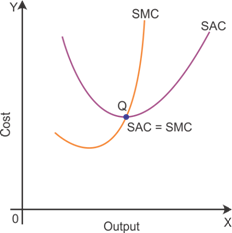
The short run marginal cost curve (SMC) cuts the short run average cost curve (SAC) from below at its minimum point (see diagram).
At the initial stage, SMC remains below SAC when there is a decline in SAC. When SAC starts increasing, SMC goes above SAC and gradually becomes more than SAC.
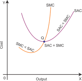
Behaviour of SAC and SMC
Solution 20
Due to the law of variable proportions, the short run marginal cost curve is U-shaped. In the short run, the output can be changed by changing the variable factors of production.
At the initial stage, an increase in the variable factors of production causes an increase in the output. At this stage, the output increases at an increasing rate.
After increasing returns to scale, there will be constant returns to scale and then eventually there will be decreasing returns to factors of production.
Solution 21
Long run marginal cost and average variable cost curves are U shaped. Law of returns to scale is the main cause of the U-shaped long run marginal cost and average cost curves. The marginal cost and average cost curves are little flatter than the shape of curves in the short run.
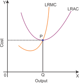
Long run marginal cost and average cost curves
Solution 22
Average product is the output per unit of variable input. The following formula can be used to describe the average product:
![]()
![]()
Marginal product of an input is the change in total output caused by the changes in the variable inputs when other inputs are held constant.
The following formula can be used to describe the marginal product of an input:
![]()
Calculation of the average product and marginal product:
|
L |
|
AP |
MP |
|
0 |
0 |
0 |
- |
|
1 |
15 |
15 |
15 |
|
2 |
35 |
17.5 |
20 |
|
3 |
50 |
16.67 |
15 |
|
4 |
40 |
10 |
-10 |
|
5 |
48 |
9.6 |
-8 |
Solution 23
Total product is the summation of final units of output produced by a firm by using the given amount of inputs during a particular period of time.
The following formula can be used to express the total product:
Total Product = ![]()
The following formula can be used to describe the marginal product of an input:
![]()
![]()
Calculation of total product and marginal product:
|
L |
|
|
|
|
1 |
2 |
2 |
2 |
|
2 |
3 |
6 |
4 |
|
3 |
4 |
12 |
6 |
|
4 |
4.25 |
17 |
5 |
|
5 |
4 |
20 |
3 |
|
6 |
3.5 |
21 |
1 |
Solution 24
The following formula can be used to calculate the total product of labour:
Total Product = ![]()
The following formula can be used to calculate the average product:
![]()
Calculation of total product and average product:
|
L |
|
|
|
|
1 |
3 |
3 |
3 |
|
2 |
5 |
8 |
4 |
|
3 |
7 |
15 |
5 |
|
4 |
5 |
20 |
5 |
|
5 |
3 |
23 |
4.60 |
|
6 |
1 |
24 |
4 |
Solution 25
The total fixed cost can be calculated by deducting the total variable cost from the total cost. Normally, the fixed cost remains the same during different levels of production.
Total variable cost is the cost incurred by producers for acquiring the variable factors of production. For example, the cost of buying labour can be considered the total variable cost. Total variable cost can be changed in the short run.
|
Q |
TC |
TFC |
TVC |
AFC |
AVC |
SAC |
SMC |
|
0 |
10 |
10 |
- |
- |
- |
- |
- |
|
1 |
30 |
10 |
20 |
10 |
20 |
30 |
20 |
|
2 |
45 |
10 |
35 |
5 |
17.5 |
22.5 |
15 |
|
3 |
55 |
10 |
45 |
3.33 |
15 |
18.33 |
10 |
|
4 |
70 |
10 |
60 |
2.5 |
15 |
17.5 |
15 |
|
5 |
90 |
10 |
80 |
2 |
16 |
18 |
20 |
|
6 |
120 |
10 |
110 |
1.66 |
18.33 |
19.99 |
30 |
Production and Costs Exercise 52
Solution 26
The total variable cost can be calculated by deducting the total fixed cost from the total cost. The total fixed cost remains the same at all output levels.
The average cost is calculated by considering the total cost and the number of inputs.
Average fixed cost is calculated by considering the number of inputs used in production and the total fixed cost.
The short marginal cost indicates the changes in total cost.
Calculation of TVC, TFC, AVC, AFC, SAC and SMC schedules of the firm.
|
Q |
TC |
TVC |
TFC |
AVC |
AFC |
SAC |
SMC |
|
1 |
50 |
30 |
20 |
30 |
20 |
50 |
30 |
|
2 |
65 |
45 |
20 |
22.5 |
10 |
32.5 |
15 |
|
3 |
75 |
55 |
20 |
27.5 |
6.66 |
34.16 |
10 |
|
4 |
95 |
75 |
20 |
18.75 |
5 |
23.75 |
20 |
|
5 |
130 |
110 |
20 |
22 |
4 |
26 |
35 |
|
6 |
185 |
165 |
20 |
27.5 |
3.33 |
30.83 |
55 |
Solution 27
The total variable cost can be calculated by deducting the total fixed cost from the total cost. The total fixed cost remains the same at all output levels. The average variable cost is calculated by considering the total variable cost and the number of inputs.
The total cost is a summation of the total variable cost and the total fixed cost.
Calculation of TVC, TC, AVC and SAC schedules of the firm:
|
Q |
SMC |
TFC |
TVC |
TC |
AVC |
SAC |
|
0 |
- |
100 |
- |
100 |
- |
- |
|
1 |
500 |
100 |
500 |
600 |
500 |
600 |
|
2 |
300 |
100 |
800 |
900 |
400 |
450 |
|
3 |
200 |
100 |
1000 |
1100 |
333.33 |
366.67 |
|
4 |
300 |
100 |
1300 |
1400 |
325 |
350 |
|
5 |
500 |
100 |
1800 |
1900 |
360 |
380 |
|
6 |
800 |
100 |
2600 |
2700 |
433.33 |
450 |
Solution 28
As given,
Capital (k) = 100 units
Labour (L) = 100 units
Applying the units of labour and capital in the equation,

Hence, the firm can produce a maximum output of 500 units.
Solution 29
As given,
Capital (k) = 2 units
Labour (L) = 5 units
Putting the units of labour and capital in the equation,

Hence, the firm can produce a maximum output of 200 units with 5 units of L and 2 units of K.
The following is a calculation of the maximum possible output that the firm can produce with zero unit of L and 10 units of K.
As given,
Capital (k) = 10 units
Labour (L) = 0 units
Putting the units of labour and capital in the equation,
Q=2(0)2 (10)2
Q = 0 units
Hence, the firm can produce a maximum output of 0 units with 0 units of L and 10 units of K.
Solution 30
As given,
Capital (k) = 10 units
Labour (L) = 0 units
Putting the units of labour and capital in the equation,

Hence, the firm can produce a maximum output of 20 units with zero units of L and 10 units of K.